Fitting with iminuit
Overview
Teaching: 15 min
Exercises: 0 minQuestions
TBD
Objectives
TBD
This episode will introduce the iminuit package for fitting data.
More information about it, as well as a host of tutorials, can be found in its documentation;
this episode draws heavily from these tutorials.
For information on fitting in the context of particle physics, see chapter 4 of Statistics for nuclear and particle physicists by Louis Lyons, from which this episode also draws.
What is a fit?
A fit is a procedure to determine some parameters of a model we want to use to describe data. Suppose we have some dataset that looks like this:
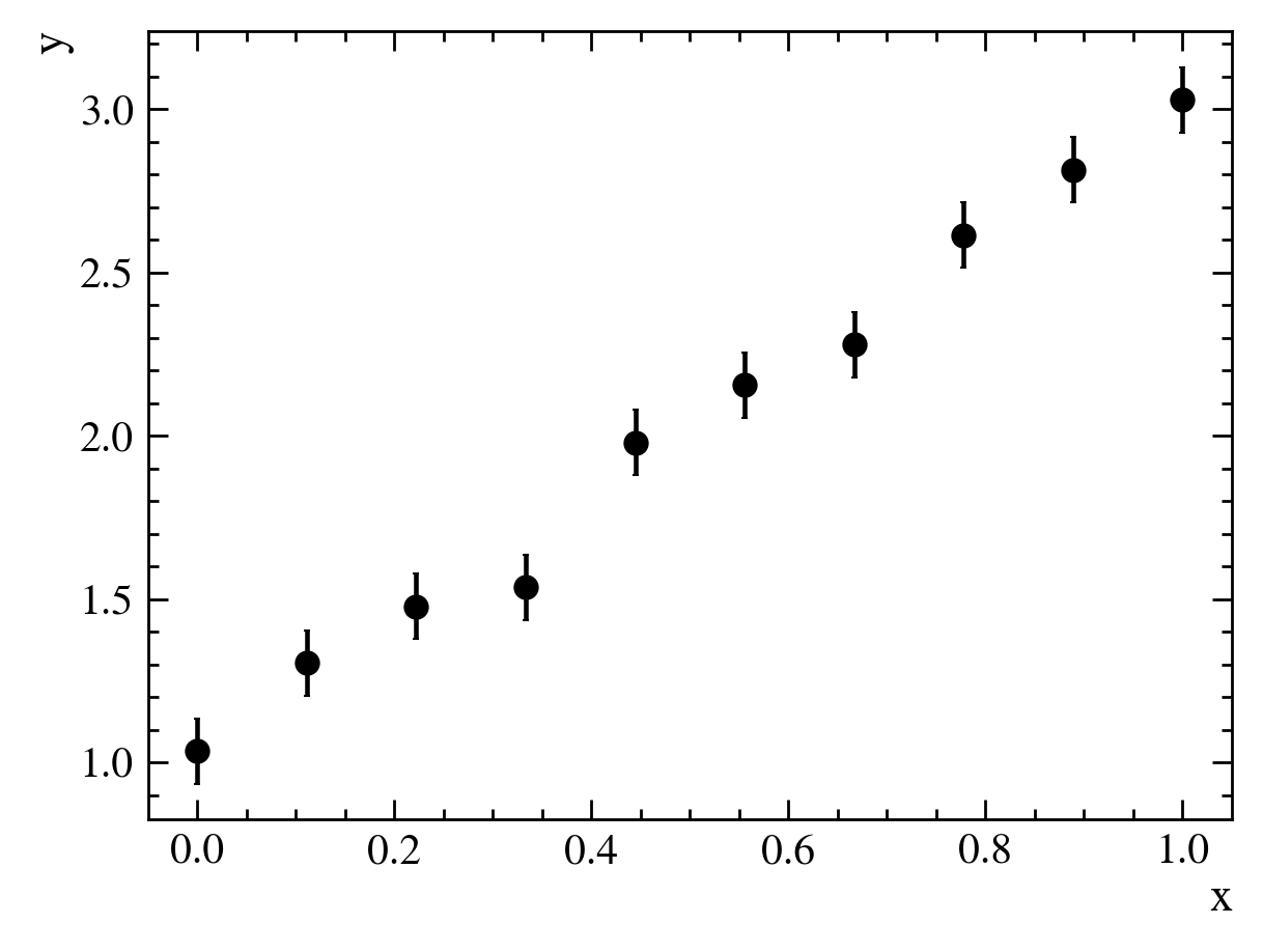
For each value of $x$, we have measured a corresponding value of $y$. We want to come up with an equation, or “model”, that describes the relationship between $x$ and $y$.
From looking at the data, it looks like a straight line, $y = f(x) \equiv mx + b$, might be a good model. In this case, $f(x,m,b)$ is our model, and it has two parameters $m$ and $b$ that we need to determine. We can do this by fitting the model to the data.
First, we need to guess some values for our parameters, say, $m=1$ and $b=0$. If we plot our model alongside our data, we see that it doesn’t fit very well:
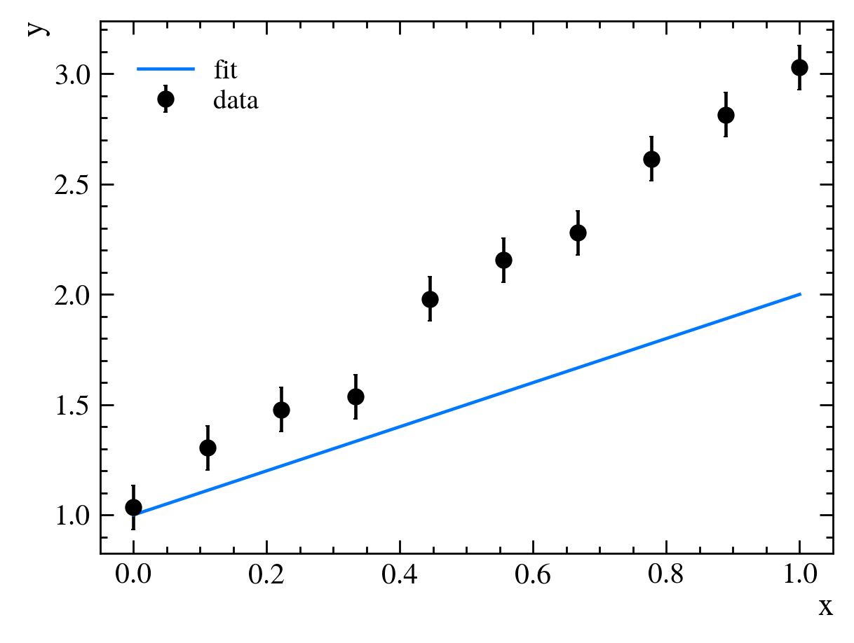
It looks like the slope of our line, $m$, is too gradual, though our y-intercept, $b$, is about right. We then adjust our parameters to get better agreement between our data and our model, setting $m=2$ and $b=0$:
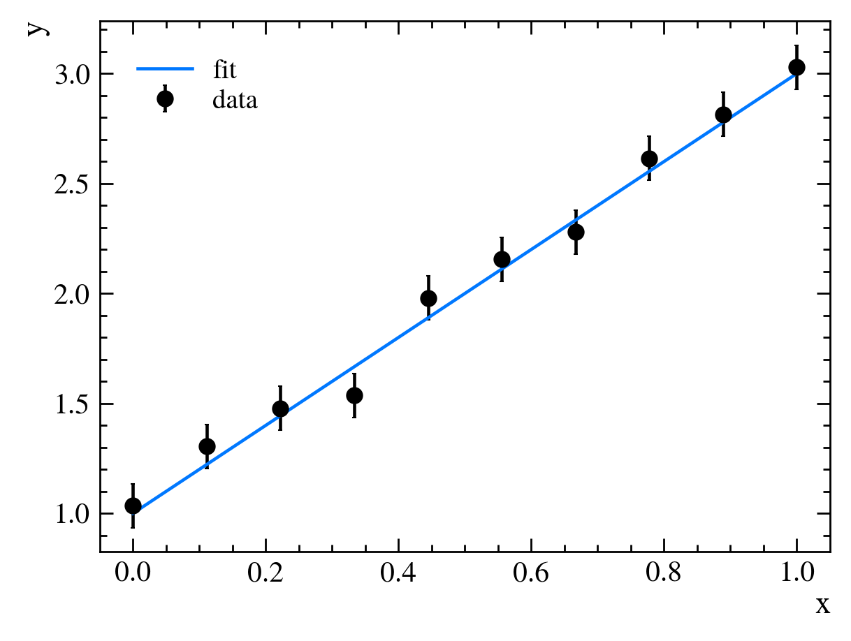
This now looks about right. We have fit our model to our data.
How good is our fit?
We performed the fit above using only qualitative evaluations of how well our model agreed with the data. We can be a bit more quantitative by defining a “goodness of fit” metric, which tells us how well our model describes the data. One such metric is the $\chi^2$ statistic, defined as \(\chi^2(\vec{\theta})=\sum_{i=1}^N\frac{(y_i-f(x_i,\vec{\theta}))^2}{\sigma_i^2},\) where $N$ is the number of measurements, $i$ is an index indicating each measurement in turn, $x_i$ indicates the $x$ value of the $i$th measurement, $y_i$ is the value measured at $x_i$, $\sigma_i$ is the uncertainty on the $i$th measurement, and $f(x_i,\vec{\theta})$ is the value of the model at $x_i$ with parameters $\vec{\theta}$. The $\chi^2$ statistic is a measure of how well our model describes the data, with smaller values indicating a better fit.
We can see this by calculating the $\chi^2$ statistic for our model above. Our measurements can be organized in a table like this:
| $i$ | $x_i$ | $y_i$ | $\sigma_i$ |
|---|---|---|---|
| 1 | 0.00 | 1.03 | 0.1 |
| 2 | 0.11 | 1.30 | 0.1 |
| 3 | 0.22 | 1.48 | 0.1 |
| 4 | 0.33 | 1.54 | 0.1 |
| 5 | 0.44 | 1.98 | 0.1 |
| 6 | 0.56 | 2.16 | 0.1 |
| 7 | 0.67 | 2.28 | 0.1 |
| 8 | 0.78 | 2.61 | 0.1 |
| 9 | 0.89 | 2.81 | 0.1 |
| 10 | 1.00 | 3.03 | 0.1 |
Our initial model was $f(x,m=1,b=1) = x + 1$. We can add that to the table above:
| $i$ | $x_i$ | $y_i$ | $\sigma_i$ | $f(x_i,m=1,b=1)$ |
|---|---|---|---|---|
| 1 | 0.00 | 1.03 | 0.1 | 1.00 |
| 2 | 0.11 | 1.30 | 0.1 | 1.11 |
| 3 | 0.22 | 1.48 | 0.1 | 1.22 |
| 4 | 0.33 | 1.54 | 0.1 | 1.33 |
| 5 | 0.44 | 1.98 | 0.1 | 1.44 |
| 6 | 0.56 | 2.16 | 0.1 | 1.56 |
| 7 | 0.67 | 2.28 | 0.1 | 1.67 |
| 8 | 0.78 | 2.61 | 0.1 | 1.78 |
| 9 | 0.89 | 2.81 | 0.1 | 1.89 |
| 10 | 1.00 | 3.03 | 0.1 | 2.00 |
Now we calculate the $\chi^2$ statistic: \(\chi^2(m=1,b=1) = \frac{(1.03-1.00)^2}{0.1^2} + \frac{(1.30-1.11)^2}{0.1^2} + \cdots + \frac{(3.03-2.00)^2}{0.1^2} = 378.\) We can compare this with our improved model, $f(x,m=2,b=1) = 2 \times x + 1$:
| $i$ | $x_i$ | $y_i$ | $\sigma_i$ | $f(x_i,m=1,b=1)$ | $f(x_i,m=2,b=1)$ |
|---|---|---|---|---|---|
| 1 | 0.00 | 1.03 | 0.1 | 1.00 | 1.00 |
| 2 | 0.11 | 1.30 | 0.1 | 1.11 | 1.22 |
| 3 | 0.22 | 1.48 | 0.1 | 1.22 | 1.44 |
| 4 | 0.33 | 1.54 | 0.1 | 1.33 | 1.67 |
| 5 | 0.44 | 1.98 | 0.1 | 1.44 | 1.89 |
| 6 | 0.56 | 2.16 | 0.1 | 1.56 | 2.11 |
| 7 | 0.67 | 2.28 | 0.1 | 1.67 | 2.33 |
| 8 | 0.78 | 2.61 | 0.1 | 1.78 | 2.56 |
| 9 | 0.89 | 2.81 | 0.1 | 1.89 | 2.78 |
| 10 | 1.00 | 3.03 | 0.1 | 2.00 | 3.00 |
and calculate the $\chi^2$ statistic: \(\chi^2(m=2,b=1) = \frac{(1.03-1.00)^2}{0.1^2} + \frac{(1.30-1.22)^2}{0.1^2} + \cdots + \frac{(3.03-3.00)^2}{0.1^2} = 4.47,\) which is much smaller than for our initial model. This confirms quantitatively what we saw qualitatively before, that our second model is a better description of the data—it “fits” better.
The method above is also called the “least squares” method of parameter determination. Technically, we can only identify it with the $\chi^2$ statistic in certain cases (including the above); since these are the cases we are most interested in, we will treat the two (“least squares” and “$\chi^2$”) as synonymous.
We typically assess the quality of the fit by looking not at the $\chi^2$ value itself, but at the “reduced $\chi^2$” value, defined as \(\chi^2_{\text{red}} \equiv \frac{\chi^2}{N_{\text{dof}}},\) where $N_{\text{dof}}$ is the number of degrees of freedom, defined as the number of measurements minus the number of parameters in the model. For the above example, $N_{\text{dof}} = 10 - 2 = 8$. The reduced $\chi^2$ value is a measure of how well our model describes the data, normalized by the number of measurements and the number of parameters in the model. A reduced $\chi^2$ value of 1 indicates a good fit, while values significantly larger than 1 indicate a poor fit. Using the reduced $\chi^2$ allows us to easily compare fit quality across models (which may have different numbers of parameters) and across datasets (which may have different numbers of measurements).
The reduced $\chi^2$ value for our first model is $\chi^2{\text{red}}(m=1,b=1) = 47.3$, a poor fit, and for our second model is $\chi^2{\text{red}}(m=2,b=1) = 0.56$, a great fit. If this were a real experiment, the second reduced $\chi^2$ is so good that we would be suspicious, as values less than 1 are unlikely and are generally a sign of over fitting; here, it is just a consequence of how we generated the data.
How can we find the best parameter values?
Above, we guessed some parameter values and picked the ones that gave us the lowest $\chi^2$, but how can we be sure that this is the lowest possible $\chi^2$? Put another way, we would like to find the parameter values that minimize the $\chi^2$ value.
(For such a simple minimization, we could find the answer analytically [by solving matrices], but for more complicated models, this is not possible, and we have to use numerical methods that involve guessing. For the purposes of illustration, we will use numerical methods below.)
To ensure we are at a minimum, we will need at least three guesses for the $\chi^2$. To keep things simple, we will only try to minimize the $\chi^2$ with respect to the $m$ parameter—we will keep $b$ fixed at 1. We then make a third guess for $m$, say $m=3$:
| $i$ | $x_i$ | $y_i$ | $\sigma_i$ | $f(x_i,m=1,b=1)$ | $f(x_i,m=2,b=1)$ | $f(x_i,m=3,b=1)$ |
|---|---|---|---|---|---|---|
| 1 | 0.00 | 1.03 | 0.1 | 1.00 | 1.00 | 1.00 |
| 2 | 0.11 | 1.30 | 0.1 | 1.11 | 1.22 | 1.33 |
| 3 | 0.22 | 1.48 | 0.1 | 1.22 | 1.44 | 1.67 |
| 4 | 0.33 | 1.54 | 0.1 | 1.33 | 1.67 | 2.00 |
| 5 | 0.44 | 1.98 | 0.1 | 1.44 | 1.89 | 2.33 |
| 6 | 0.56 | 2.16 | 0.1 | 1.56 | 2.11 | 2.67 |
| 7 | 0.67 | 2.28 | 0.1 | 1.67 | 2.33 | 3.00 |
| 8 | 0.78 | 2.61 | 0.1 | 1.78 | 2.56 | 3.33 |
| 9 | 0.89 | 2.81 | 0.1 | 1.89 | 2.78 | 3.67 |
| 10 | 1.00 | 3.03 | 0.1 | 2.00 | 3.00 | 4.00 |
and calculate the $\chi^2$ statistic, $\chi^2 = 334$. We can now plot the $\chi^2$ values for our three guesses:
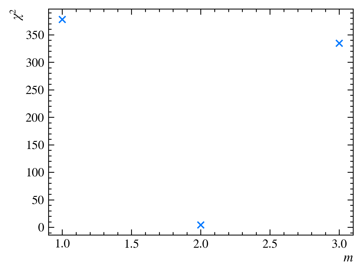
It looks like the $\chi^2_{\text{red}}$ value does have a minimum between $m=1$ and $m=3$, possibly at $m=2$. To find it exactly, we can draw a parabola that crosses the three points:
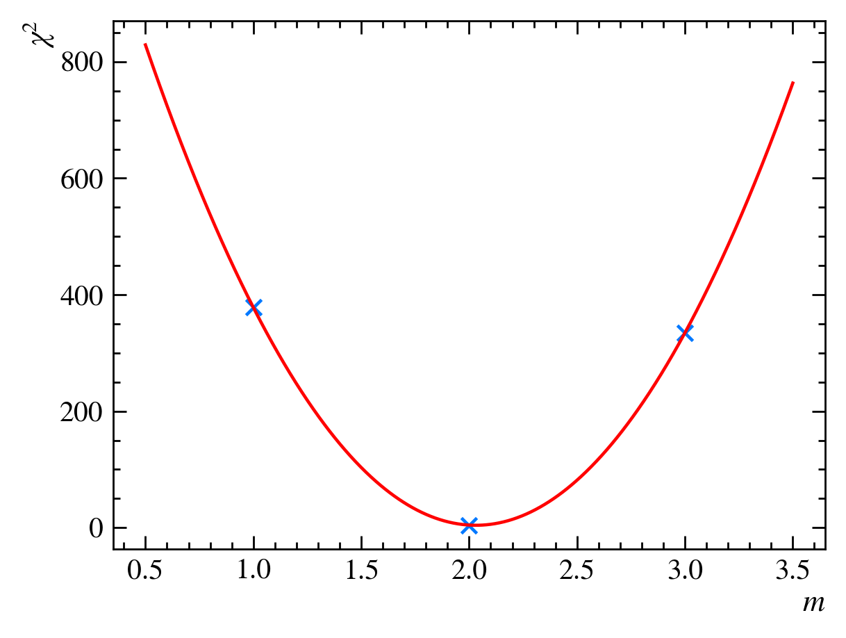
We then calculate the minimum of the parabola to be at $m=m_0=2.03$. If we calculate the reduced $\chi^2$ value for this guess, we find $\chi^2{\text{red}}(m=2.03,b=1) = 0.52$, which is slightly better than our previous best guess, $\chi^2{\text{red}}(m=2,b=1) = 0.56$. We have now minimized our $\chi^2$ as a function of $m$:
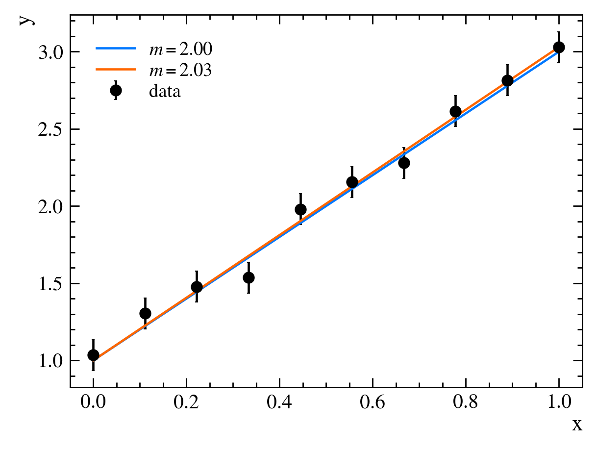
How confident are we that this is the best value of $m$? We can calculate an error for our minimized value based on the width of the parabola, which we determine by finding the value of $m$ at $\text{min}(\chi^2) + 1$ and taking the absolute difference between this value and $m_0$:
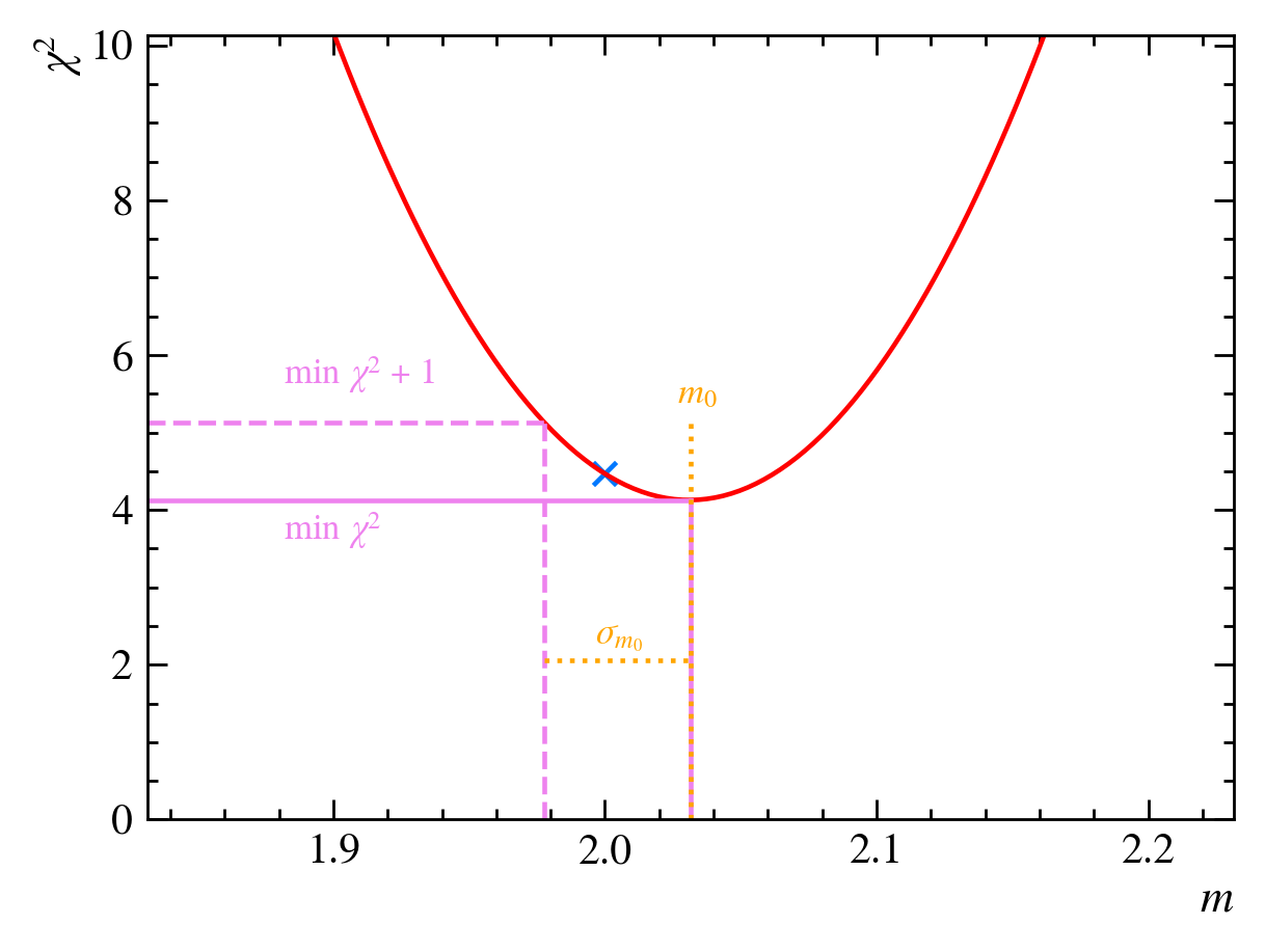
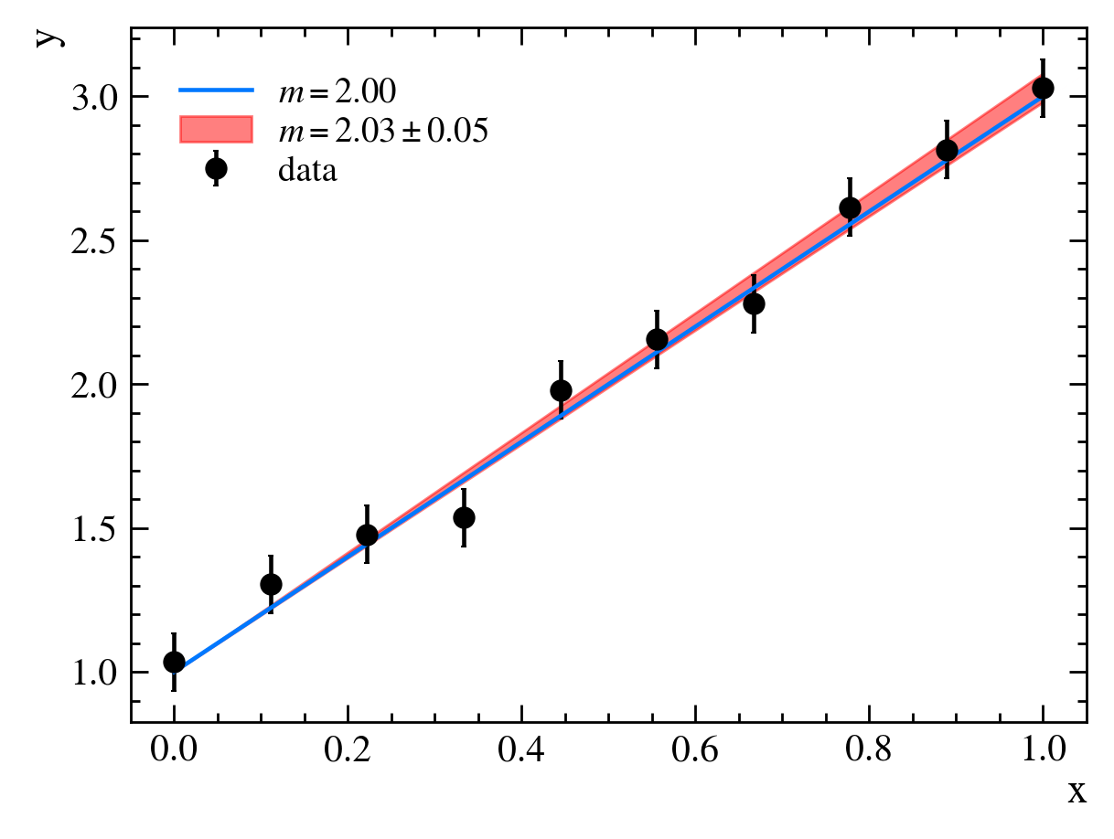
In our case, we find $m=2.03 \pm 0.05$:
Choosing trial parameters
In the above example, we chose $m=1$, $m=2$, and $m=3$ as our trial values based on how our model appeared to align with the data in the plot. This was fine for our simple example here, but for more complicated models, we would want to define an algorithmic way of determining which parameter values to guess.
One such algorithm is called “gradient descent”, which involves taking the derivative of the $\chi^2$ function with respect to the parameters to be minimized and adjusting them in the direction of smaller $\chi^2$ values. Another algorithm is called “Newton’s method”, which involves adjusting parameter values based on second-derivatives. A discussion of these algorithms is beyond the scope of this episode, but they will be used behind the scenes when we start with the iminuit package below.
Is this really the minimum?
We have certainly found a minimum for $\chi^2(m)$, but is it the minimum? How can we be sure there is not another, lower value of the $\chi^2$ somewhere else that we did not check? Well, for simple minimization problems with analytical solutions, like the one above, we could have solved for the minimum explicitly, but for more complicated models, this may not be possible. In these cases, we won’t be sure that we have really found the absolute “global” minimum, only that we have found a “local” one (or something close to it)—the only way to be really sure would be to check every possible value for the parameters, which we can’t do with finite computing resources. It is therefore important to start our minimization from a reasonable location by choosing appropriate guesses for our parameters; this helps give us confidence that we have arrived at an appropriate solution.
What is iminuit?
iminuit is a Jupyter-friendly python interface to Minuit2, a piece of software written in C++ that combines a minimizer (MIGRAD) and error calculators (HESSE and MINOS). It takes an analytical function, which has several parameters, and a guess for the initial parameter values; it then finds a local minimum of this function. It can also compute uncertainty estimates for the parameters.
Let’s use iminuit to repeat the fit process above. First, let us generate the same dataset as before:
# our line model
import numpy as np

def line(x, b, m):
    return b + m * x

# generate random toy data with random offsets in y
rng = np.random.default_rng(1)
data_x = np.linspace(0, 1, 10)
data_yerr = 0.1  # could also be an array
data_y = rng.normal(line(data_x, 1, 2), data_yerr)
Now, we could define our own $\chi^2$ function and minimize it using iminuit, but iminuit includes a number of cost functions, including LeastSquares, which, as we said above, is effectively another name for the $\chi^2$ function in our case. We import it from iminuit.cost and then tell it to use our dataset and model:
from iminuit.cost import LeastSquares

least_squares = LeastSquares(data_x, data_y, data_yerr, line)
The iminuit docs include a tutorial on cost functions that goes into more detail on how to use them.
Now we can perform the minimization:
# minimization in iminuit is handled through the Minuit class, so we import it
from iminuit import Minuit

# we then initialize the minimizer
# this does not actually perform any minimization yet, just makes sure it is set up properly
# notice that we can pass it starting values for our parameters by name
m = Minuit(least_squares, m=1, b=1)

# now we perform the minimization
m.migrad()  # minimizes least_squares
m.hesse()  # computes the parameter uncertainties
This should produce output like the following:
| Migrad | |
|---|---|
| FCN = 3.959 (χ²/ndof = 0.5) | Nfcn = 42 |
| EDM = 5.56e-21 (Goal: 0.0002) | |
| Valid Minimum | Below EDM threshold (goal x 10) |
| No parameters at limit | Below call limit |
| Hesse ok | Covariance accurate |
| Name | Value | Hesse Error | Minos Error- | Minos Error+ | Limit- | Limit+ | Fixed | |
|---|---|---|---|---|---|---|---|---|
| 0 | b | 1.02 | 0.06 | |||||
| 1 | m | 2.0 | 0.1 |
| b | m | |
|---|---|---|
| b | 0.00345 | -0.0049 (-0.843) |
| m | -0.0049 (-0.843) | 0.00982 |
<?xml version=”1.0” encoding=”utf-8” standalone=”no”?> <!DOCTYPE svg PUBLIC “-//W3C//DTD SVG 1.1//EN” “http://www.w3.org/Graphics/SVG/1.1/DTD/svg11.dtd”>
Key Points
TBD